Shortcuts in ODE and SDE

TLDR

In the context of generative modeling, we examine ODEs, SDEs, and two recent works that share the idea of learning shortcuts that traverse through vector fields defined by ODEs faster. We then discuss the generalization of this idea to both ODE- and SDE-based models.

Differential Equations

Let’s start with a general scenario of generative modeling: suppose you want to generate data $x$ that follows a distribution $p(x)$. In many cases, the exact form of $p(x)$ is unknown. What you can do is follow the idea of normalizing flow¹: start from a very simple, closed-form distribution $p(x_0)$ (for example, a standard normal distribution), transform this distribution through time $t\in [0,1]$ with intermediate distributions $p(x_t)$, and finally obtain the estimated distribution $p(x_1)$. By doing this, you are essentially trying to solve a differential equation (DE)² that depends on time:

$$d{x}_t=\mu (x_t,t)dt+\sigma (x_t,t)d{W}_t,x_0\sim p(x_0)$$

where $\mu$ is the drift component that is deterministic, and $\sigma$ is the diffusion term driven by Brownian motion³ (denoted by $W_t$) that is stochastic. This differential equation specifies a time-dependent vector (velocity) field⁴ telling how a data point $x_t$ should be moved as time $t$ evolves from $t=0$ to $t=1$ (i.e., a flow⁵ from $x_0$ to $x_1$). Below we give an illustration where $x_t$ is 1-dimensional:

Vector field between two distributions specified by a differential equation.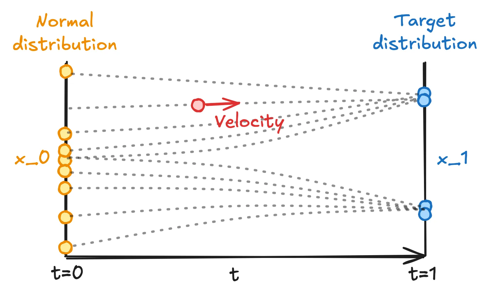

When $\sigma (x_t,t)\equiv 0$, we get an ordinary differential equation (ODE)⁶ where the vector field is deterministic, i.e., the movement of $x_t$ is fully determined by $\mu$ and $t$. Otherwise, we get a stochastic differential equation (SDE)⁷ where the movement of $x_t$ has a certain level of randomness. Extending the previous illustration, below we show the difference in flow of $x_t$ under ODE and SDE:

Difference of movements in vector fields specified by ODE and SDE. Source: Song, Yang, et al. “Score-based generative modeling through stochastic differential equations.” Note that their time is reversed.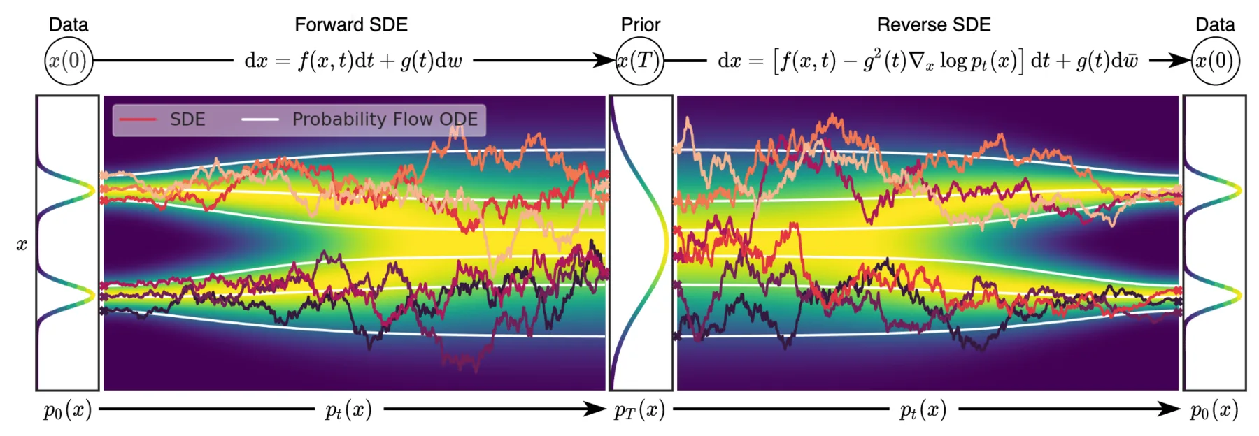

As you would imagine, once we manage to solve the differential equation, even if we still cannot have a closed form of $p(x_1)$, we can sample from $p(x_1)$ by sampling a data point $x_0$ from $p(x_0)$ and get the generated data point $x_1$ by calculating the following forward-time integral with an integration technique of our choice:

$$x_1=x_0+{\int }_0^1\mu (x_t,t)dt+{\int }_0^1\sigma (x_t,t)d{W}_t$$

Or more intuitively, moving $x_0$ towards $x_1$ along time in the vector field:

A flow of data point moving from $x_0$ towards $x_1$ in the vector field.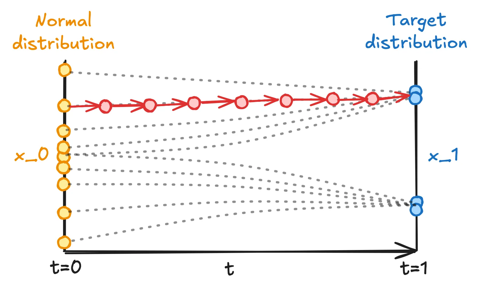

ODE and Flow Matching

ODE in Generative Modeling

For now, let’s focus on the ODE formulation since it is notationally simpler compared to SDE. Recall the ODE of our generative model:

$$\frac{d{x}_t}{dt}=\mu (x_t,t)$$

Essentially, $\mu$ is the vector field. For every possible combination of data point $x_t$ and time $t$, $\mu (x_t,t)$ is the instantaneous velocity in which the point will move. To generate a data point $x_1$, we perform the integral:

$$x_1=x_0+{\int }_0^1\mu (x_t,t)dt$$

To calculate this integral, a simple and widely adopted method is the Euler method⁸. Choose $N$ time steps $0=t_0<t_1<\cdots <t_{N-1}<t_N=1$, and for each integral step $k=0,1,\dots ,N-1$:

$$x_{t_{k+1}}=x_{t_k}+(t_{k+1}-t_k)\mu (x_{t_k},t_k)$$

In other words, we discretize the time span $[0,1]$ into $N$ time steps, and for each step the data is moved based on the instantaneous velocity at the current step.

Note

There are other methods to calculate the integral, of course. For example, one can use the solvers in the torchdiffeq Python package⁹.

Flow Matching

In many scenarios, the exact form of the vector field $\mu$ is unknown. The general idea of flow matching¹⁰ is to find a ground truth vector field that defines the flow transporting $p(x_0)$ to $p(x_1)$, and build a neural network ${\mu }_{\theta }$ that is trained to match the ground truth vector field, hence the name. In practice, this is usually done by independently sampling $x_0$ from the noise and $x_1$ from the training data, calculating the intermediate data point $x_t$ and the ground truth velocity $\mu (x_t,t)$, and minimizing the deviation between ${\mu }_{\theta }(x_t,t)$ and $\mu (x_t,t)$.

Ideally, the ground truth vector field should be as straight as possible, so we can use a small number of $N$ steps to calculate the ODE integral. Thus, the ground truth velocity is usually defined following the optimal transport flow map:

$$x_t=t{x}_1+(1-t)x_0,\mu (x_t,t)=x_1-x_0$$

And a neural network ${\mu }_{\theta }$ is trained to match the ground truth vectors as:

$$\mathcal{L}={\mathbb{E}}_{x_0,x_1,t}\Vert {\mu }_{\theta }(x_t,t)-(x_1-x_0){\Vert }^2$$

Curvy Vector Field

Although the ground truth vector field is designed to be straight, in practice it usually is not. When the data space is high-dimensional and the target distribution $p(x_1)$ is complex, there will be multiple pairs of $(x_0,x_1)$ that result in the same intermediate data point $x_t$, thus multiple velocities $x_1-x_0$. At the end of the day, the actual ground truth velocity at $x_t$ will be the average of all possible velocities $x_1-x_0$ that pass through $x_t$. This will lead to a “curvy” vector field, illustrated as follows:

Left: multiple vectors passing through the same intermediate data point. Right: the resulting ground truth vector field. Source: Geng, Zhengyang, et al. “Mean Flows for One-step Generative Modeling.” Note $z_t$ and $v$ in the figure correspond to $x_t$ and $\mu$ in this post, respectively.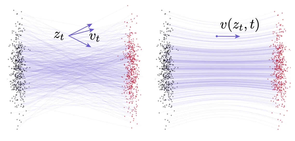

As we discussed, when you calculate the ODE integral, you are using the instantaneous velocity—tangent of the curves in the vector field—of each step. You would imagine this will lead to subpar performance when using a small number $N$ of steps, as demonstrated below:

Native flow matching models fail at few-step sampling. Source: Frans, Kevin, et al. “One step diffusion via shortcut models.”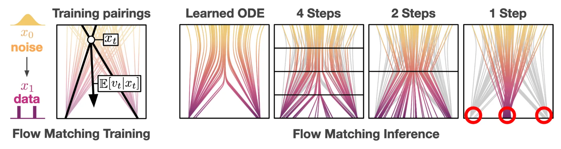

Shortcut Vector Field

If we cannot straighten the ground truth vector field, can we tackle the problem of few-step sampling by learning velocities that properly jump across long time steps instead of learning the instantaneous velocities? Yes, we can.

Shortcut Models

Shortcut models¹¹ implement the above idea by training a network $u_{\theta }(x_t,t,\Delta t)$ to match the velocities that jump across long time steps (termed shortcuts in the paper). A ground truth shortcut $u(x_t,t,\Delta t)$ will be the velocity pointing from $x_t$ to $x_{t+\Delta t}$, formally:

$$u(x_t,t,\Delta t)=\frac{1}{\Delta t}{\int }_t^{t+\Delta t}\mu (x_{\tau },\tau )d\tau$$

Ideally, you can transform $x_0$ to $x_1$ within one step with the learned shortcuts:

$$x_1\approx x_0+u_{\theta }(x_0,0,1)$$

Note

Of course, in practice shortcut models face the same problem mentioned in the Curvy Vector Field: the same data point $x_1$ corresponds to multiple shortcut velocities to different data points $x_0$, making the ground truth shortcut velocity at $x_1$ the average of all possibilities. So, shortcut models have a performance advantage with few sampling steps compared to conventional flow matching models, but typically don’t have the same performance with one step versus more steps.

The theory is quite straightforward. The tricky part is in the model training. First, the network expands from learning all possibilities of velocities at $(x_t,t)$ to all velocities at $(x_t,t,\Delta t)$ with $\Delta t\in [0,t]$. Essentially, the shortcut vector field has one more dimension than the instantaneous vector field, making the learning space larger. Second, calculating the ground truth shortcut involves calculating integral, which can be computationally heavy.

To tackle these challenges, shortcut models introduce self-consistency shortcuts: one shortcut with step size $2\Delta t$ should equal two consecutive shortcuts both with step size $\Delta t$:

$$u(x_t,t,2\Delta t)=u(x_t,t,\Delta t)/2+u(x_{t+\Delta t},t+\Delta t,\Delta t)/2$$

The model is then trained with the combination of matching instantaneous velocities and self-consistency shortcuts as below. Notice that we don’t train a separate network for matching the instantaneous vectors but leverage the fact that the shortcut $u(x_t,t,\Delta t)$ is the instantaneous velocity when $\Delta t\to 0$.

$$\mathcal{L}={\mathbb{E}}_{x_0,x_1,t,\Delta t}[\underset{\text{Flow-Matching}}{\underbrace{\Vert u_{\theta }(x_t,t,0)-(x_1-x_0){\Vert }^2}}+\underset{\text{Self-Consistency}}{\underbrace{\Vert u_{\theta }(x_t,t,2\Delta t)-\text{sg}({\mathbf{u}}_{\text{target}}){\Vert }^2}}],$$ $${\mathbf{u}}_{\text{target}}=u_{\theta }(x_t,t,\Delta t)/2+u_{\theta }(x_{t+\Delta t}^{\prime },t+\Delta t,\Delta t)/2\text{and}{x}_{t+\Delta t}^{\prime }=x_t+\Delta t\cdot u_{\theta }(x_t,t,\Delta t)$$

Where $\text{sg}$ is stop gradient, i.e., detach ${\mathbf{u}}_{\text{target}}$ from back propagation, making it a pseudo ground truth. Below is an illustration of the training process provided in the original paper.

Training of the shortcut models with self-consistency loss.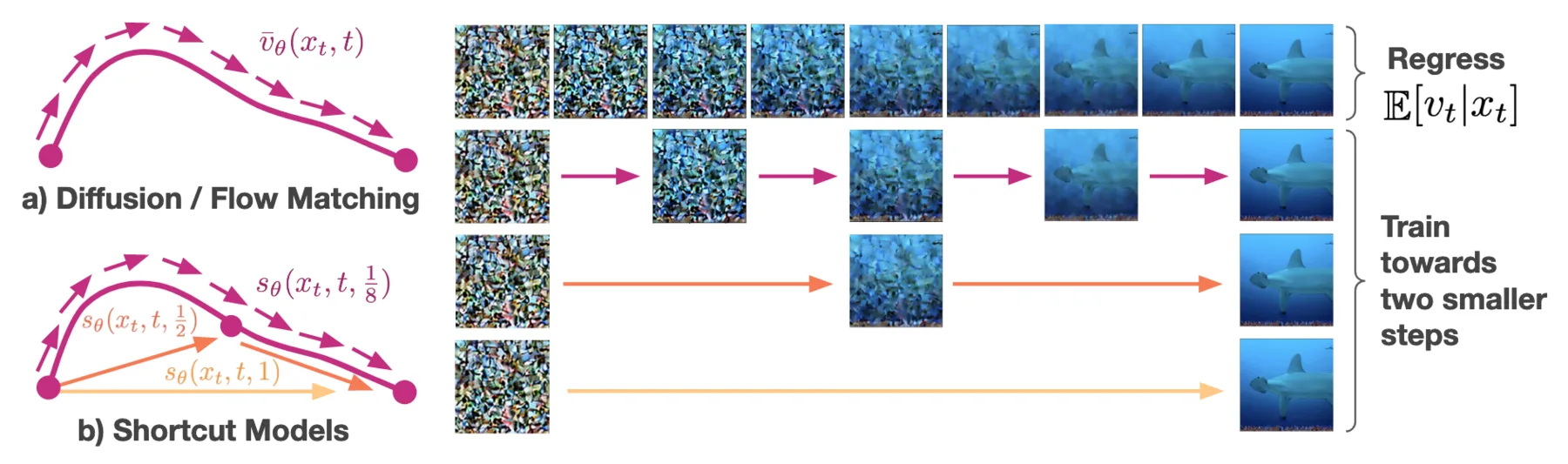

Mean Flow

Mean flow¹² is another work sharing the idea of learning velocities that take large step size shortcuts but with a stronger theoretical foundation and a different approach to training.

Illustration of the average velocity provided in the original paper.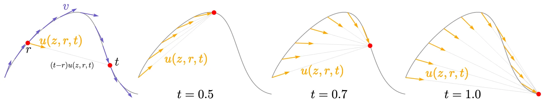

Mean flow defines an average velocity as a shortcut between times $t$ and $r$ where $t$ and $r$ are independent:

$$u(x_t,r,t)=\frac{1}{t-r}{\int }_r^t\mu (x_{\tau },\tau )d\tau$$

This average velocity is essentially equivalent to a shortcut in shortcut models given $\Delta t=t-r$. What differentiates mean flow from shortcut models is that mean flow aims to provide a ground truth of the vector field defined by $u(x_t,r,t)$, and directly train a network $u_{\theta }(x_t,r,t)$ to match the ground truth.

We transform the above equation by differentiate both sides with respect to $t$ and rearrange components, and get:

$$u(x_t,r,t)=\mu (x_t,t)+(r-t)\frac{d}{dt}u(x_t,r,t)$$

We get the average velocity on the left, and the instantaneous velocity and the time derivative components on the right. This defines the ground truth average vector field, and our goal now is to calculate the right side. We already know that the ground truth instantaneous velocity $\mu (x_t,t)=x_1-x_0$. To compute the time derivative component, we can expand it in terms of partial derivatives:

$$\frac{d}{dt}u(x_t,r,t)=\frac{d{x}_t}{dt}{\partial }_{x}u+\frac{dr}{dt}{\partial }_{r}u+\frac{dt}{dt}{\partial }_{t}u$$

From the ODE definition $d{x}_t/dt=\mu (x_t,t)$, and $dt/dt=1$. Since $t$ and $r$ are independent, $dr/dt=0$. Thus, we have:

$$\frac{d}{dt}u(x_t,r,t)=\mu (x_t,t){\partial }_{x}u+{\partial }_{t}u$$

This means the time derivative component is the vector product between $[{\partial }_{x}u,{\partial }_{r}u,{\partial }_{t}u]$ and $[\mu ,0,1]$. In practice, this can be computed using the Jacobian vector product (JVP) functions in NN libraries, such as the torch.func.jvp function in PyTorch. In summary, the mean flow loss function is:

$$\mathcal{L}={\mathbb{E}}_{x_t,r,t}\Vert u_{\theta }(x_t,r,t)-\text{sg}(\mu (x_t,t)+(r-t)(\mu (x_t,t){\partial }_x{u}_{\theta }+{\partial }_t{u}_{\theta })){\Vert }^2$$

Notice that the JVP computation inside $\text{sg}$ is performed with the network $u_{\theta }$ itself. In this regard, this loss function shares a similar idea with the self-consistency loss in shortcut models—supervising the network with output produced by the network itself.

Extended Reading: Rectified Flow

Both shortcut models and mean flow are built on top of the ground truth curvy ODE field. They don’t modify the field $\mu$, but rather try to learn shortcut velocities that can traverse the field with fewer Euler steps. This is reflected in their loss function design: shortcut models’ loss function specifically includes a standard flow matching component, and mean flow’s loss function is derived from the relationship between vector fields $\mu$ and $u$.

Rectified flow¹³, another family of flow matching models that aims to achieve one-step sampling, is fundamentally different in this regard. It aims to replace the original ground truth ODE field with a new one with straight flows. Ideally, the resulting ODE field has zero curvature, enabling one-step integration with the simple Euler method. This usually involves augmentation of the training data and a repeated reflow process.

We won’t discuss rectified flow in further detail in this post, but it’s worth pointing out its difference from shortcut models and mean flow.

SDE and Score Matching

SDE in Generative Modeling

SDE, as its name suggests, is a differential equation with a stochastic component. Recall the general differential equation we introduced at the beginning:

$$d{x}_t=\mu (x_t,t)dt+\sigma (x_t,t)d{W}_t$$

In practice, the diffusion term $\sigma$ usually only depends on $t$, so we will use the simpler formula going forward:

$$d{x}_t=\mu (x_t,t)dt+\sigma (t)d{W}_t$$

$W_t$ is the Brownian motion (a.k.a. standard Wiener process). In practice, its behavior over time $t$ can be described as $W_{t+\Delta t}-W_t\sim \mathcal{N}(0,\Delta t)$. This is the source of SDE’s stochasticity, and also why people like to call the family of SDE-based generative models diffusion models¹⁴, since Brownian motion is derived from physical diffusion processes¹⁵.

In the context of generative modeling, the stochasticity in SDE means it can theoretically handle augmented data or data that is stochastic in nature (e.g., financial data) more gracefully. Practically, it also enables techniques such as stochastic control guidance¹⁶. At the same time, it also means SDE is mathematically more complicated compared to ODE. We no longer have a deterministic vector field $\mu$ specifying flows of data points $x_0$ moving towards $x_1$. Instead, both $\mu$ and $\sigma$ have to be designed to ensure that the SDE leads to the target distribution $p(x_1)$ we want.

To solve the SDE, similar to the Euler method used for solving ODE, we can use the Euler-Maruyama method¹⁷:

$$x_{t_{k+1}}=x_{t_k}+(t_{k+1}-t_k)\mu (x_t,t)+\sqrt{t_{k+1}-t_k}\sigma (t)ϵ,ϵ\sim \mathcal{N}(0,1)$$

In other words, we move the data point guided by the velocity $\mu (x_t,t)$ plus a bit of Gaussian noise scaled by $\sqrt{t_{k+1}-t_k}\sigma (t)$.

Score Matching

In SDE, the exact form of the vector field $\mu$ is still (quite likely) unknown. To solve this, the general idea is consistent with flow matching: we want to find the ground truth $\mu (x_t,t)$ and build a neural network ${\mu }_{\theta }(x_t,t)$ to match it.

Score matching models¹⁸ implement this idea by parameterizing $\mu$ as:

$$\mu (x_t,t)=v(x_t,t)+\frac{{\sigma }^2(t)}{2}\nabla \log p(x_t)$$

where $v(x_t,t)$ is a velocity similar to that in ODE, and $\nabla \log p(x_t)$ is the score (a.k.a. informant)¹⁹ of $x_t$. Without going too deep into the relevant theories, think of the score as a “compass” that points in the direction where $x_t$ becomes more likely to belong to the distribution $p(x_1)$. The beauty of introducing the score is that depending on the definition of ground truth $x_t$, the velocity $v$ can be derived from the score, or vice versa. Then, we only have to focus on building a learnable score function $s_{\theta }(x_t,t)$ to match the ground truth score using the loss function below, hence the name score matching:

$$\mathcal{L}={\mathbb{E}}_{x_t,t}\Vert s_{\theta }(x_t,t)-\nabla \log p(x_t){\Vert }^2$$

For example, if we have time-dependent coefficients ${\alpha }_t$ and ${\beta }_t$ (termed noise schedulers in most diffusion models), and define that $x_t$ follows the distribution given a clean data point $x_1$:

$$p(x_t)=\mathcal{N}({\alpha }_t{x}_1,{\beta }_t^2)$$

then we will have:

$$\nabla \log p(x_t)=-\frac{x_t-{\alpha }_t{x}_1}{{\beta }_t^2},v(x_t,t)=\left({\beta }_t^2\frac{{\partial }_t{\alpha }_t}{{\alpha }_t}-({\partial }_t{\beta }_t){\beta }_t\right)\nabla \log p(x_t)+\frac{{\partial }_t{\alpha }_t}{{\alpha }_t}{x}_t$$

Some works¹⁴ also propose to re-parameterize the score function with noise $ϵ$ sampled from a standard normal distribution, so that the neural network can be a learnable denoiser ${ϵ}_{\theta }(x_t,t)$ that matches the noise rather than the score. Since $s_{\theta }=-{ϵ}_{\theta }/\sigma (t)$, both approaches are equivalent.

Shortcuts in SDE

Most existing efforts sharing the idea of shortcut vector fields are grounded in ODEs. However, given the correlations between SDE and ODE, learning an SDE that follows the same idea should be straightforward. Generally speaking, SDE training, similar to ODE, focuses on the deterministic drift component $\mu$. One should be able to, for example, use the same mean flow loss function to train a score function for solving an SDE.

Note

Needless to say, generalizing shortcut models and mean flow to flow matching models with ground truth vector fields other than optimal transport flow requires no modification either, since most such models (e.g., Bayesian flow) are ultimately grounded in ODE.

One caveat of training a “shortcut SDE” is that the ideal result of one-step sampling contradicts the stochastic nature of SDE—if you are going to perform the sampling in one step, you are probably better off using ODE to begin with. Still, I believe it would be useful to train an SDE so that its benefits versus ODE are preserved, while still enabling the lowering of sampling steps $N$ for improved computational efficiency.

Below are some preliminary results I obtained from a set of amorphous material generation experiments. You don’t need to understand the figure—just know that it shows that applying the idea of learning shortcuts to SDE does yield better results compared to the vanilla SDE when using few-step sampling.

Structural functions of generated materials, sampled in 10 steps.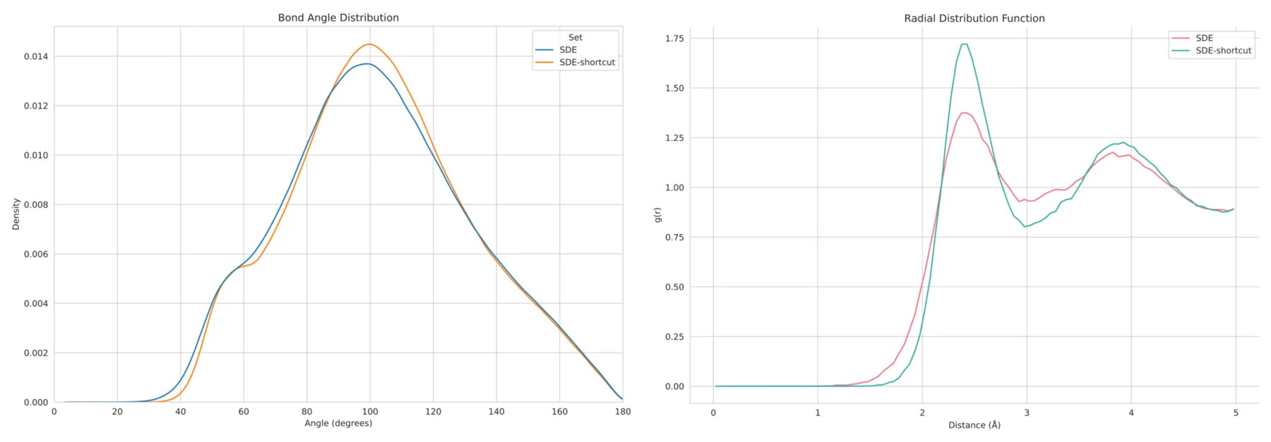

---

References

• Holderrieth and Erives, “An Introduction to Flow Matching and Diffusion Models.”
• Song and Ermon, “Generative Modeling by Estimating Gradients of the Data Distribution.”

Footnotes

1. Rezende, Danilo, and Shakir Mohamed. “Variational inference with normalizing flows.” ↩

2. https://en.wikipedia.org/wiki/Differential_equation ↩

3. https://en.wikipedia.org/wiki/Brownian_motion ↩

4. https://en.wikipedia.org/wiki/Vector_field ↩

5. https://en.wikipedia.org/wiki/Vector_flow ↩

6. https://en.wikipedia.org/wiki/Ordinary_differential_equation ↩

7. https://en.wikipedia.org/wiki/Stochastic_differential_equation ↩

8. https://en.wikipedia.org/wiki/Euler_method ↩

9. https://github.com/rtqichen/torchdiffeq ↩

10. Lipman, Yaron, et al. “Flow matching for generative modeling.” ↩

11. Frans, Kevin, et al. “One step diffusion via shortcut models. ↩

12. Geng, Zhengyang, et al. “Mean Flows for One-step Generative Modeling.” ↩

13. Flow Straight and Fast: Learning to Generate and Transfer Data with Rectified Flow ↩

14. Ho, Jonathan, Ajay Jain, and Pieter Abbeel. “Denoising diffusion probabilistic models.” ↩ ↩²

15. https://en.wikipedia.org/wiki/Diffusion_process ↩

16. Huang et al., “Symbolic Music Generation with Non-Differentiable Rule Guided Diffusion.” ↩

17. https://en.wikipedia.org/wiki/Euler–Maruyama_method ↩

18. Song et al., “Score-Based Generative Modeling through Stochastic Differential Equations.” ↩

19. https://en.wikipedia.org/wiki/Informant_(statistics) ↩